Partial and total derivatives on computation graphs

Rich Pang

2025-10-22

Some clarifications about derivatives on computation graphs. This extends Christopher Olah's excellent post about this topic and is meant to help make sense of different factorizations of loss gradients, e.g. in the e-prop algorithm of Bellec et al 2020.

Partial derivatives and Jacobians

The partial derivative describes how a function changes with respect to one of its arguments. A crucial observation is that the partial derivative depends on how the functions in question are specified. For instance, consider case 1 where we write \[z = x^2 + y^2\] \[L = z^2 + x^2\] vs case 2 where we write \[L = 2x^2 + y^2,\]

which describe the same relationship between \(L\) and \(x\). However, in case 1 \[\frac{\partial L}{\partial x} = 2x\] whereas in case 2 \[\frac{\partial L}{\partial x} = 4x.\] Thus when talking about the partial derivative of one variable computed through a series of intermediate steps from several other variables, one needs to be precise about what those intermediate steps are.

The Jacobian of a function, specifically a vector-valued function of multiple arguments, is the matrix of partial derivatives of each component of the function value with respect to each argument. For instance, suppose

\[\mathbf{y} = \mathbf{y}(\mathbf{x})\]

where \(\mathbf{x} \in \mathbb{R}^n\) and \(\mathbf{y} \in \mathbb{R}^m\). Then the Jacobian \(\mathcal{D}_{\mathbf{y}\mathbf{x}}\) is

\[\mathcal{D}_{\mathbf{y}\mathbf{x}} = \begin{bmatrix} \dfrac{\partial y_1}{\partial x_1} & \cdots & \dfrac{\partial y_1}{\partial x_n} \\ \vdots & \ddots & \vdots \\ \dfrac{\partial y_m}{\partial x_1} & \cdots & \dfrac{\partial y_m}{\partial x_n} \end{bmatrix}\]

Paths on computation graphs

Computation graphs are visual representations of a series of steps used to compute a function value. Suppose a loss \(L\) is computed from \(w\) in the following way:

\[\mathbf{x} = \mathbf{x}(\mathbf{w})\]

\[\mathbf{y} = \mathbf{y}(\mathbf{x}, \mathbf{w})\]

\[\mathbf{z} = \mathbf{z}(\mathbf{y}, \mathbf{w})\]

\[L = L(\mathbf{x}, \mathbf{y}, \mathbf{z}).\]

This series of functions and dependencies can be represented as

Computation graphs are a fundamental abstraction in modern AI, and understanding them is essential to understanding the computation of gradients.

Of frequent interest are paths on computation graphs. When we speak of the path from \(\mathbf{w}\) to \(\mathbf{x}\) to \(\mathbf{y}\) to \(L\), what we are actually referring to is the product of Jacobians backwards along that path:

\[\mathcal{D}_{L\mathbf{y}} \mathcal{D}_{\mathbf{y}\mathbf{x}} \mathcal{D}_{\mathbf{x}\mathbf{w}}.\]

The path conveys the flow of information from the source variable, \(\mathbf{w}\) to the target variable \(L\). This can be useful for intuiting about e.g. vanishing gradients. A long path, for instance, often corresponds to a large number of Jacobians with eigenvalues less than 1, whose product vanishes. Hence a small change in the source variable will lead to no change in the target variable, at least through that particular path.

Total derivatives

The total derivative of a target variable with respect to a source variable is the sum of all possible ways a small change in the source will lead to a small change in the target. On the computation graph above, the total derivative of \(dL/d\mathbf{x}\) corresponds to the sum of all (directed) paths from \(\mathbf{x}\) to \(L\). That is, \(dL/d\mathbf{x}\) corresponds to:

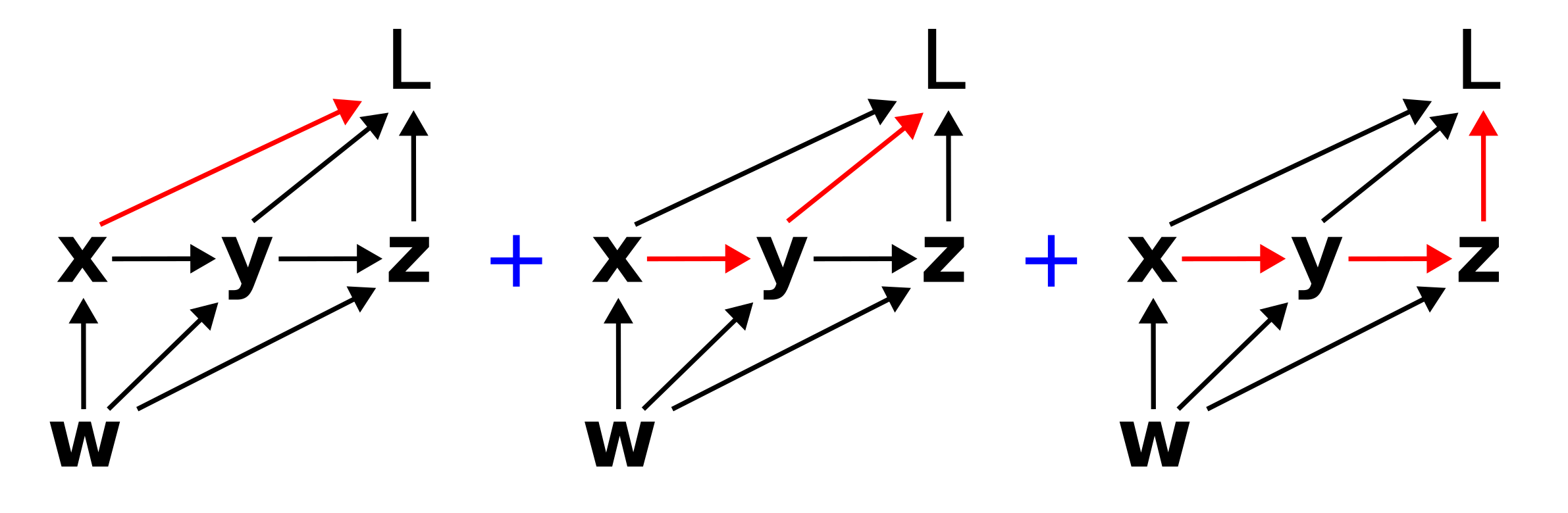
Not that the paths can overlap, e.g. multiple paths can include the same edge (link). Mathematically, this sum corresponds to

\[\frac{dL}{d\mathbf{x}} = \mathcal{D}_{L\mathbf{x}} + \mathcal{D}_{L\mathbf{y}}\mathcal{D}_{\mathbf{y}\mathbf{x}} + \mathcal{D}_{L\mathbf{z}}\mathcal{D}_{\mathbf{z}\mathbf{y}}\mathcal{D}_{\mathbf{y}\mathbf{x}}.\]

Similarly \(dL/d\mathbf{w}\) would correspond to the sum of all six paths from \(\mathbf{w}\) to \(L\).

Factorizing paths

Summing over paths can be a tricky combinatorics problem, and it can be useful to think about different ways to factorize the sum. The key point is to look for common terms. For instance, the sum

\[\frac{dL}{d\mathbf{w}} = \mathcal{D}_{L\mathbf{x}}\mathcal{D}_{\mathbf{x}\mathbf{w}} + \mathcal{D}_{L\mathbf{y}}\mathcal{D}_{\mathbf{y}\mathbf{x}}\mathcal{D}_{\mathbf{x}\mathbf{w}} + \mathcal{D}_{L\mathbf{z}}\mathcal{D}_{\mathbf{z}\mathbf{y}}\mathcal{D}_{\mathbf{y}\mathbf{x}}\mathcal{D}_{\mathbf{x}\mathbf{w}}\]

\[+ \mathcal{D}_{L\mathbf{y}}\mathcal{D}_{\mathbf{y}\mathbf{w}} + \mathcal{D}_{L\mathbf{z}}\mathcal{D}_{L\mathbf{y}}\mathcal{D}_{\mathbf{y}\mathbf{w}} + \mathcal{D}_{L\mathbf{z}}\mathcal{D}_{\mathbf{z}\mathbf{w}}\]

can be factorized as

\[\frac{dL}{d\mathbf{w}} = \left(\mathcal{D}_{L\mathbf{x}} + \mathcal{D}_{L\mathbf{y}}\mathcal{D}_{\mathbf{y}\mathbf{x}} + \mathcal{D}_{L\mathbf{z}}\mathcal{D}_{\mathbf{z}\mathbf{y}}\mathcal{D}_{\mathbf{y}\mathbf{x}}\right)\mathcal{D}_{\mathbf{x}\mathbf{w}}\]

\[+ \left( \mathcal{D}_{L\mathbf{y}} + \mathcal{D}_{L\mathbf{z}}\mathcal{D}_{L\mathbf{y}} \right) \mathcal{D}_{\mathbf{y}\mathbf{w}} + \mathcal{D}_{L\mathbf{z}}\mathcal{D}_{\mathbf{z}\mathbf{w}},\]

which is quite a bit more palatable, and interestingly equivalent to

\[\frac{dL}{d\mathbf{w}} = \frac{dL}{d\mathbf{x}}\mathcal{D}_{\mathbf{x}\mathbf{w}} + \frac{dL}{d\mathbf{y}}\mathcal{D}_{\mathbf{y}\mathbf{w}} + \frac{dL}{d\mathbf{z}}\mathcal{D}_{\mathbf{z}\mathbf{w}}.\]

In upcoming posts we will talk about the classical factorization of back-propagation through time, as well as the e-prop factorization.

Special thanks to Helena Liu for proofreading this post.